Standard ContainersA container is a holder object that stores a collection of other objects (its elements). They are implemented as class templates, which allows a great flexibility in the types supported as elements.

The container manages the storage space for its elements and provides member functions to access them, either directly or through iterators (reference objects with similar properties to pointers).

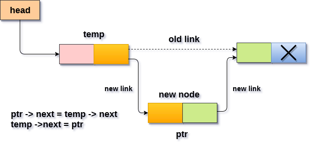
Containers replicate structures very commonly used in programming: dynamic arrays (vector), queues (queue), stacks (stack), heaps (priority_queue), linked lists (list), trees (set), associative arrays (map)…

Many containers have several member functions in common, and share functionalities. The decision of which type of container to use for a specific need does not generally depend only on the functionality offered by the container, but also on the efficiency of some of its members (complexity). This is especially true for sequence containers, which offer different trade-offs in complexity between inserting/removing elements and accessing them.

stack, queue and priority_queue are implemented as container adaptors. Container adaptors are not full container classes, but classes that provide a specific interface relying on an object of one of the container classes (such as deque or list) to handle the elements. The underlying container is encapsulated in such a way that its elements are accessed by the members of the container adaptor independently of the underlying container class used.

Container class templates

Sequence containers:
array Array class (class template )vectorVector (class template )dequeDouble ended queue (class template )forward_list Forward list (class template )listList (class template )
Container adaptors:
stackLIFO stack (class template )queueFIFO queue (class template )priority_queuePriority queue (class template )
Associative containers:
setSet (class template )multisetMultiple-key set (class template )mapMap (class template )multimapMultiple-key map (class template )
Unordered associative containers:
unordered_set Unordered Set (class template )unordered_multiset Unordered Multiset (class template )unordered_map Unordered Map (class template )unordered_multimap Unordered Multimap (class template )
Other:
Two class templates share certain properties with containers, and are sometimes classified with them: bitset and valarray.

Member map

This is a comparison chart with the different member functions present on each of the different containers:

Legend:

C++98	Available since C++98
C++11	New in C++11

Sequence containers

Headers	<array>	<vector>	<deque>	<forward_list>	<list>
Members	array	vector	deque	forward_list	list
	constructor	implicit	vector	deque	forward_list	list
destructor	implicit	~vector	~deque	~forward_list	~list
operator=	implicit	operator=	operator=	operator=	operator=
iterators	begin	begin	begin	begin	begin before_begin	begin
end	end	end	end	end	end
rbegin	rbegin	rbegin	rbegin		rbegin
rend	rend	rend	rend		rend
const iterators	cbegin	cbegin	cbegin	cbegin	cbegin cbefore_begin	cbegin
cend	cend	cend	cend	cend	cend
crbegin	crbegin	crbegin	crbegin		crbegin
crend	crend	crend	crend		crend
capacity	size	size	size	size		size
max_size	max_size	max_size	max_size	max_size	max_size
empty	empty	empty	empty	empty	empty
resize		resize	resize	resize	resize
shrink_to_fit		shrink_to_fit	shrink_to_fit
capacity		capacity
reserve		reserve
element access	front	front	front	front	front	front
back	back	back	back		back
operator[]	operator[]	operator[]	operator[]
at	at	at	at
modifiers	assign		assign	assign	assign	assign
emplace		emplace	emplace	emplace_after	emplace
insert		insert	insert	insert_after	insert
erase		erase	erase	erase_after	erase
emplace_back		emplace_back	emplace_back		emplace_back
push_back		push_back	push_back		push_back
pop_back		pop_back	pop_back		pop_back
emplace_front			emplace_front	emplace_front	emplace_front
push_front			push_front	push_front	push_front
pop_front			pop_front	pop_front	pop_front
clear		clear	clear	clear	clear
swap	swap	swap	swap	swap	swap
list operations	splice				splice_after	splice
remove				remove	remove
remove_if				remove_if	remove_if
unique				unique	unique
merge				merge	merge
sort				sort	sort
reverse				reverse	reverse
observers	get_allocator		get_allocator	get_allocator	get_allocator	get_allocator
data	data	data

Associative containers

Headers	<set>	<map>	<unordered_set>	<unordered_map>
Members	set	multiset	map	multimap	unordered_set	unordered_multiset	unordered_map	unordered_multimap
	constructor	set	multiset	map	multimap	unordered_set	unordered_multiset	unordered_map	unordered_multimap
destructor	~set	~multiset	~map	~multimap	~unordered_set	~unordered_multiset	~unordered_map	~unordered_multimap
assignment	operator=	operator=	operator=	operator=	operator=	operator=	operator=	operator=
iterators	begin	begin	begin	begin	begin	begin	begin	begin	begin
end	end	end	end	end	end	end	end	end
rbegin	rbegin	rbegin	rbegin	rbegin
rend	rend	rend	rend	rend
const iterators	cbegin	cbegin	cbegin	cbegin	cbegin	cbegin	cbegin	cbegin	cbegin
cend	cend	cend	cend	cend	cend	cend	cend	cend
crbegin	crbegin	crbegin	crbegin	crbegin
crend	crend	crend	crend	crend
capacity	size	size	size	size	size	size	size	size	size
max_size	max_size	max_size	max_size	max_size	max_size	max_size	max_size	max_size
empty	empty	empty	empty	empty	empty	empty	empty	empty
reserve					reserve	reserve	reserve	reserve
element access	at			at				at
operator[]			operator[]				operator[]
modifiers	emplace	emplace	emplace	emplace	emplace	emplace	emplace	emplace	emplace
emplace_hint	emplace_hint	emplace_hint	emplace_hint	emplace_hint	emplace_hint	emplace_hint	emplace_hint	emplace_hint
insert	insert	insert	insert	insert	insert	insert	insert	insert
erase	erase	erase	erase	erase	erase	erase	erase	erase
clear	clear	clear	clear	clear	clear	clear	clear	clear
swap	swap	swap	swap	swap	swap	swap	swap	swap
operations	count	count	count	count	count	count	count	count	count
find	find	find	find	find	find	find	find	find
equal_range	equal_range	equal_range	equal_range	equal_range	equal_range	equal_range	equal_range	equal_range
lower_bound	lower_bound	lower_bound	lower_bound	lower_bound
upper_bound	upper_bound	upper_bound	upper_bound	upper_bound
observers	get_allocator	get_allocator	get_allocator	get_allocator	get_allocator	get_allocator	get_allocator	get_allocator	get_allocator
key_comp	key_comp	key_comp	key_comp	key_comp
value_comp	value_comp	value_comp	value_comp	value_comp
key_eq					key_eq	key_eq	key_eq	key_eq
hash_function					hash_function	hash_function	hash_function	hash_function
buckets	bucket					bucket	bucket	bucket	bucket
bucket_count					bucket_count	bucket_count	bucket_count	bucket_count
bucket_size					bucket_size	bucket_size	bucket_size	bucket_size
max_bucket_count					max_bucket_count	max_bucket_count	max_bucket_count	max_bucket_count
hash policy	rehash					rehash	rehash	rehash	rehash
load_factor					load_factor	load_factor	load_factor	load_factor
max_load_factor					max_load_factor	max_load_factor	max_load_factor	max_load_factor

 Linear Search Algorithm | Example | Time Complexity

Searching-

• Searching is a process of finding a particular element among several given elements.
• The search is successful if the required element is found.
• Otherwise, the search is unsuccessful.

Searching Algorithms-

Searching Algorithms are a family of algorithms used for the purpose of searching.

The searching of an element in the given array may be carried out in the following two ways-

1. Linear Search
2. Binary Search

In this article, we will discuss about Linear Search Algorithm

Linear Search-

• Linear Search is the simplest searching algorithm.
• It traverses the array sequentially to locate the required element.
• It searches for an element by comparing it with each element of the array one by one.
• So, it is also called as Sequential Search.

Linear Search Algorithm is applied when-

• No information is given about the array.
• The given array is unsorted or the elements are unordered.
• The list of data items is smaller.

Linear Search Algorithm-

Consider-

• There is a linear array ‘a’ of size ‘n’.
• Linear search algorithm is being used to search an element ‘item’ in this linear array.
• If search ends in success, it sets loc to the index of the element otherwise it sets loc to -1.

Then, Linear Search Algorithm is as follows-

Linear_Search (a , n , item , loc)

Begin

for i = 0 to (n – 1) by 1 do

if (a[i] = item) then

set loc = i

Exit

endif

end for

set loc = -1

End

Time Complexity Analysis-

Linear Search time complexity analysis is done below-

Best case-

In the best possible case,

• The element being searched may be found at the first position.
• In this case, the search terminates in success with just one comparison.
• Thus in best case, linear search algorithm takes O(1) operations.

Worst Case-

In the worst possible case,

• The element being searched may be present at the last position or not present in the array at all.
• In the former case, the search terminates in success with n comparisons.
• In the later case, the search terminates in failure with n comparisons.
• Thus in worst case, linear search algorithm takes O(n) operations.

Thus, we have-

Linear Search Efficiency-

• Linear Search is less efficient when compared with other algorithms like Binary Search & Hash tables.
• The other algorithms allow significantly faster searching.

Linear Search Example-

Consider-

• We are given the following linear array.
• Element 15 has to be searched in it using Linear Search Algorithm.

Now,

• Linear Search algorithm compares element 15 with all the elements of the array one by one.
• It continues searching until either the element 15 is found or all the elements are searched.

Linear Search Algorithm works in the following steps-

Step-01:

• It compares element 15 with the 1st element 92.
• Since 15 ≠ 92, so required element is not found.
• So, it moves to the next element.

Step-02:

• It compares element 15 with the 2nd element 87.
• Since 15 ≠ 87, so required element is not found.
• So, it moves to the next element.

Step-03:

• It compares element 15 with the 3rd element 53.
• Since 15 ≠ 53, so required element is not found.
• So, it moves to the next element.

Step-04:

• It compares element 15 with the 4th element 10.
• Since 15 ≠ 10, so required element is not found.
• So, it moves to the next element.

Step-05:

• It compares element 15 with the 5th element 15.
• Since 15 = 15, so required element is found.
• Now, it stops the comparison and returns index 4 at which element 15 is present

1.insert an element after a given
element.

In order to insert an element after the specified number of nodes into the linked list, we need to skip the desired number of elements in the list to move the pointer at the position after which the node will be inserted. This will be done by using the following statements.

1. emp=head;  
2.             for(i=0;i<loc;i++)  
3.             {  
4.                 temp = temp->next;  
5.                 if(temp == NULL)  
6.                 {  
7.                     return;  
8.                 }  
9.               
10.             } 

• Allocate the space for the new node and add the item to the data part of it. This will be done by using the following statements.

1. ptr = (struct node *) malloc (sizeof(struct node));  
2.         ptr->data = item;  

• Now, we just need to make a few more link adjustments and our node at will be inserted at the specified position. Since, at the end of the loop, the loop pointer temp would be pointing to the node after which the new node will be inserted. Therefore, the next part of the new node ptr must contain the address of the next part of the temp (since, ptr will be in between temp and the next of the temp). This will be done by using the following statements.

1. ptr→ next = temp → next   

now, we just need to make the next part of the temp, point to the new node ptr. This will insert the new node ptr, at the specified position.

1. temp ->next = ptr;   

Algorithm

• STEP 1: IF PTR = NULL
• STEP 2: SET NEW_NODE = PTR
• STEP 3: NEW_NODE → DATA = VAL
• STEP 4: SET TEMP = HEAD
• STEP 5: SET I = 0
• STEP 6: REPEAT STEP 5 AND 6 UNTIL I
• STEP 7: TEMP = TEMP → NEXT
• STEP 8: IF TEMP = NULL
• STEP 9: PTR → NEXT = TEMP → NEXT
• STEP 10: TEMP → NEXT = PTR
• STEP 11: SET PTR = NEW_NODE
• STEP 12: EXIT

C Function

1. #include<stdio.h>  
2. #include<stdlib.h>  
3. void randominsert(int);  
4. void create(int);  
5. struct node  
6. {  
7.     int data;  
8.     struct node *next;  
9. };  
10. struct node *head;  
11. void main ()  
12. {  
13.     int choice,item,loc;  
14.     do   
15.     {  
16.         printf("\nEnter the item which you want to insert?\n");  
17.         scanf("%d",&item);  
18.         if(head == NULL)  
19.         {  
20.             create(item);  
21.         }  
22.         else  
23.         {  
24.             randominsert(item);  
25.         }  
26.         printf("\nPress 0 to insert more ?\n");  
27.         scanf("%d",&choice);  
28.     }while(choice == 0);  
29. }  
30. void create(int item)  
31. {  
32.       
33.         struct node *ptr = (struct node *)malloc(sizeof(struct node *));  
34.         if(ptr == NULL)  
35.         {  
36.             printf("\nOVERFLOW\n");  
37.         }  
38.         else  
39.         {  
40.             ptr->data = item;  
41.             ptr->next = head;  
42.             head = ptr;  
43.             printf("\nNode inserted\n");  
44.         }  
45. }  
46. void randominsert(int item)  
47.     {  
48.         struct node *ptr = (struct node *) malloc (sizeof(struct node));  
49.         struct node *temp;  
50.         int i,loc;  
51.         if(ptr == NULL)  
52.         {  
53.             printf("\nOVERFLOW");  
54.         }  
55.         else  
56.         {  
57.               
58.             printf("Enter the location");  
59.             scanf("%d",&loc);             
60.             ptr->data = item;  
61.             temp=head;  
62.             for(i=0;i<loc;i++)  
63.             {  
64.                 temp = temp->next;  
65.                 if(temp == NULL)  
66.                 {  
67.                     printf("\ncan't insert\n");  
68.                     return;  
69.                 }  
70.               
71.             }  
72.             ptr ->next = temp ->next;   
73.             temp ->next = ptr;   
74.             printf("\nNode inserted");  
75.         }  
76.           
77.     }  

Output

Enter the item which you want to insert?
12

Node inserted

Press 0 to insert more ?
2

 

Time-division multiplexing (TDM)

Time-division multiplexing (TDM) is a method of putting multiple data streams in a single signal by separating the signal into many segments, each having a very short duration. Each individual data stream is reassembled at the receiving end based on the timing.

The circuit that combines signals at the source (transmitting) end of a communications link is known as a multiplexer. It accepts the input from each individual end user, breaks each signal into segments, and assigns the segments to the composite signal in a rotating, repeating sequence. The composite signal thus contains data from multiple senders. At the other end of the long-distance cable, the individual signals are separated out by means of a circuit called a demultiplexer, and routed to the proper end users. A two-way communications circuit requires a multiplexer/demultiplexer at each end of the long-distance, high-bandwidth cable.

If many signals must be sent along a single long-distance line, careful engineering is required to ensure that the system will perform properly. An asset of TDM is its flexibility. The scheme allows for variation in the number of signals being sent along the line, and constantly adjusts the time intervals to make optimum use of the available bandwidth. The Internet is a classic example of a communications network in which the volume of traffic can change drastically from hour to hour. In some systems, a different scheme, known as frequency-division multiplexing (FDM), is preferred.

Applications of TDM

The first TDM was developed for telegraphy application. Using this system, multiple data transmission were routed over a single transmission line. Nowadays TDM is used for many applications which are given below.

1. TDM is used in digital audio mixing system.

2. TDM or Time Division Multiplexing is used in Pulse Code Modulation(PCM) transmission system.

3. In the optical data transmission system or optical fiber communication, Time Division Multiplexing mostly used.

4. Time Division Multiplexing or TDM is used in SONET(Synchronous Optical Networking)

5. Time Division Multiplexing or TDM is used in landline phone system such as Signaling System 7 or SS7. Here up to 24 separate phone calls or phone conservation can be multiplexed and demultiplexed.

6. In Half Duplex Communication system, TDM or Time Division Multiplexing is used.

7. Time Division Multiplexing is used in Integrated Service Digital Network or ISDN telephone system.

8. TDM also used in Public Switched Telephone Network or PSTN system.

9. TDM is used in Synchronous Digital Hierarchy or SDH system.

10. TDM is used in GSM or Global System for Mobile communication technology.

11. TDM is used in Satelite Acess system.

12. TDM is used in Cellular Radio.

 

Disadvantages of TDM

1. TDM needs synchronization but FDM does not need synchronization. It is a disadvantage of TDM over FDM.
2. Another noticeable disadvantage of TDM is that TDM provides less latency than FDM. 
3. In Time Division Multiplexing system, address information and buffer is needed.

 

 Ques- What is the significance of the following TCP header fields:

• Urgent Pointer
• Checksum
• Window Size
• Reserved bits
• Sequence Number

Ans- In the Transmission Control Protocol (TCP) Segment Header lesson, you will learn more about TCP Segment Header, different fields in TCP Header and the use of these fields.

Transmission Control Protocol (TCP) Segment Header.

Sequence number

32 Bit number used for byte level numbering of TCP segments. If you are using TCP, each byte of data is assigned a sequence number. If SYN flag is set (during the initial three way handshake connection initiation), then this is the initial sequence number. The sequence number of the actual first data byte will then be this sequence number plus 1. For example, let the first byte of data by a device in a particular TCP header will have its sequence number in this field 50000. If this packet has 500 bytes of data in it, then the next packet sent by this device will have the sequence number of 50000 500 1 = 50501.

Reserved Bits

• These bits are not used.
• The 6 bits are reserved.

Window size

Indicates the size of the receive window, which specifies the number of bytes beyond the sequence number in the acknowledgment field that the receiver is currently willing to receive.

• Thus, window size is used for Flow Control.
• It advertises how much data (in bytes) the sender can receive without acknowledgement.
• It contains the size of the receiving window of the sender.
• Window size is a 16 bit field.

Checksum

• Receiver rejects the data that fails the CRC check.
• Sender adds CRC checksum to the checksum field before sending the data.
• It verifies the integrity of data in the TCP payload.
• Checksum is a 16 bit field used for error control.

Urgent Pointer

Shows the end of the urgent data so that interrupted data streams can continue. When the URG bit is set, the data is given priority over other data streams (Size 16 bits).

Subnetting

Subnetting is the practice of dividing a network into two or more smaller networks. It increases routing efficiency, enhances the security of the network and reduces the size of the broadcast domain.

Consider the following example:

In the picture above we have one huge network: 10.0.0.0/24. All hosts on the network are in the same subnet, which has the following disadvantages:

organizational problems – in a large networks, different departments are usually grouped into different subnets. For example, you can group all devices from the Accounting department in the same subnet and then give access to sensitive financial data only to hosts from that subnet.

network security – each device can reach any other device on the network, which can present security problems. For example, a server containing sensitive information shouldn’t be in the same network as user’s workstations.

a single broadcast domain – all hosts are in the same broadcast domain. A broadcast sent by any device on the network will be processed by all hosts, creating lots of unnecessary traffic.

Subnet mask

An IP address is divided into two parts: network and host parts. For example, an IP class A address consists of 8 bits identifying the network and 24 bits identifying the host. This is because the default subnet mask for a class A IP address is 8 bits long. (or, written in dotted decimal notation, 255.0.0.0). What does it mean? Well, like an IP address, a subnet mask also consists of 32 bits. Computers use it to determine the network part and the host part of an address. The 1s in the subnet mask represent a network part, the 0s a host part.

Computers works only with bits. The math used to determine a network range is binary AND.

Let’s say that we have the IP address of 10.0.0.1 with the default subnet mask of 8 bits (255.0.0.0).
First, we need to convert the IP address to binary:

IP address: 10.0.0.1 = 00001010.00000000.00000000.00000001
Subnet mask 255.0.0.0 = 11111111.00000000.00000000.0000000

Computers then use the AND operation to determine the network number:

The computer can then determine the size of the network. Only IP addresses that begins with 10 will be in the same network. So, in this case, the range of addresses in this network is 10.0.0.0 – 10.255.255.255.

NOTE
A subnet mask must always be a series of 1s followed by a series of 0s.

DEFAULT subnet mask

By now you should have some idea what the subnet mask does and how it's used to partition a network. What you need to keep in mind is that each Class has its DEFAULT subnet mask, which we can change to suit our needs. I have already mentioned this in the previous page, but we need to look into it in a bit more detail.

 IP address is an address having information about how to reach a specific host, especially outside the LAN. An IP address is a 32 bit unique address having an address space of 232. Generally, there are two notations in which IP address is written, dotted decimal notation and hexadecimal notation.

Classful Addressing

In Classful addressing, the address space is divided into five classes: A, B, C, D, and E. Each of these classes has a valid range of IP addresses. Classes D and E are reserved for multicast and experimental purposes respectively. The order of bits in the first octet determine the classes of IP address.

IPv4 address is divided into two parts:

 

• Network ID
• Host ID

 

The class of IP address is used to determine the bits used for network ID and host ID and the number of total networks and hosts possible in that particular class. Each ISP or network administrator assigns an IP address to each device that is connected to its network.

 

 

Note: While finding the total number of host IP addresses, 2 IP addresses are not counted and are, therefore, decreased from the total count because the first IP address of any network is the network number and whereas the last IP address is reserved for broadcast IP.

The Classful addressing wastes a large part of the address space.

• Class A: 0----2^7---- 2^24
• Class B: 10--- 2^14--- 2^16
• Class C: 110---- 2^21--- 2^8
• Class D: 1110---1------ 2^28

 

Problems with Classful Addressing: 

The problem with this classful addressing method is that millions of class A address are wasted, many of the class B address are wasted, whereas, number of addresses available in class C is so small that it cannot cater the needs of organizations. Class D addresses are used for multicast routing and are therefore available as a single block only. Class E addresses are reserved. 
Since there are these problems, Classful networking was replaced by Classless Inter-Domain Routing (CIDR) in 1993.